Text Classification with Logistic Regression

Introduction

Logistics regression is a well known statistics tool for classification including text. The steps to implement a text classifier with this statistic tool will be explained here.

Training Flow

flowchart LR
    A[Text] --> B["Feature_Extraction(T)"]
    B --> C["Prediction_Function(X)"]
    C --> D["Output Y^"]
    D --> E["Cost_Function(Y, Y^)"]
    E --> C

Vocabulary & Feature Extraction

One-Hot-Encoding

Consists of creating a vector of 0s and 1s (no other values) where each position represents a word in the vocabulary. If a word is present in a phrase (such a Twit) the corresponding position would be marked as 1 otherwise 0.

Problem: Long training and prediction time: It can get too big and sparse when a large vocabulary from many different texts are used.

Negative and Positive Frequencies

The idea is to use feature vectors to count word frequencies for each prediction category (such as positive/negative in sentiment analysis). Global feature vector is calculated for each word, following the steps below:

Map(word) —> occurrence of that word in a given class

	I	am	happy	sad	never
Positive	2	2	1	0	0
Negative	3	3	0	2	1

Preprocessing

tokenization - break text into array of words
```
from nltk.tokenize import TweetTokenizer
```

stop words - eliminate meaningless words (punctuation, articles, prepositions, not-important symbols, etc.)

from nltk.corpus import stopwords
import string
nltk.download(‘stopwords’)
stopwords_english = stopwords.words(‘english’)
punctuation = string.punctuation

stemming - map word to its root form (remove ing, ed, etc.)

from nltk.stem import PorterStemmer
stemmer = PorterStemmer()
stemmed_text = [ ]
for word in text:
stem_word = stemmer.stem(word)
stemmed_text.append(stem_word)

lowercase - convert all words to lowercase

Logistics Regression

Logistics is, in essence, linear regression with sigmoid function (\(\sigma\)).

\(h(z) = \frac{1}{1 + e^{-z}}\) with \(z = \theta^T x\)

\(\sigma(x_0 \theta_0 + x_1 \theta_1 + x_2 \theta_2 + x_3 \theta_3)\)

Training Workflow

flowchart TD
    A["Theta"] --> B["h = h(X, Theta)"]
    B --> C["Nabla = 1/m X^t (h - y)"]
    C --> D["Theta = Theta - Alpha Nabla"]
    D --> E["J(Theta)"]
    E --> B

Legend:

\(\theta\) = Theta
\(\alpha\) = Alpha
\(\nabla\) = Nabla

flowchart TD
    A["Initialize parameters"] --> B["Classify/predict"]
    B --> C["Get gradient"]
    C --> D["Update"]
    D --> E["Get Loss"]
    E --> B

Testing (with accuracy)

Testing can be done via cross-validation data with \(X_{val}\), \(Y_{val}\) and \(\theta\) on the model to optimize hyper-parameters.

\(X_{val} Y_{val} \theta\)
- \(h(X_{val} . \theta)\)
- \(pred = h(X_{val} . \theta) >= 0.5\)

\[ \begin{bmatrix} 0.3 \\ 0.8 \\ 0.5 \\ \vdots \\ h_m \end{bmatrix} >= 0.5 = \begin{bmatrix} 0.3 > 0.5 \\ 0.8 > 0.5 \\ 0.5 > 0.5\\ \vdots \\ pred_m > 0.5 \end{bmatrix} = \begin{bmatrix} 0 \\ 1 \\ 1 \\ \vdots \\ pred_m \end{bmatrix} \]

\[ Accuracy \rightarrow \sum_{i=1}^{m} \frac{ (pred^{(i)} == y_{val}^{(i)}) }{m} \]

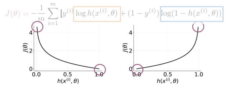
Cost Function

Makes use of a cost function J composed by 2 parts: * left part (yellow) is relevant when \(y(i) == 1\) * right part (blue) is relevant when \(y(i) == 0\)

\[ J(\theta) = - \frac{1}{m} \sum_{i=1}^{m} log(h(x^{(i)}, \theta)) + (1 - y^{(i)}) log(1 - h(x^{(i)}, \theta)) \]

Gradient Calculation (Optimization)

Gradient is calculated to adjust logistics-regression parameters during training (see flow below):

\[ Repeat \{ \theta_j = \theta_j - \alpha \frac{\partial }{\partial \theta_j} J(\theta) \} \]

For all \(j\), calculate derivatives:

\[ Repeat \{ \theta_j = \theta_j - \frac{\alpha}{m} \sum_{i=1}^{m} (h(x^{(i)}, \theta) - y^{(i)}) x_j^{(i)} \} \]

Derivative calculation can be summarized as: (with vectors)

\[ \theta = \theta - \frac{\alpha}{m} X^{T} (H(X, \theta) - Y) \]

With cost function as:

\[ \partial J(\theta) = \frac{1}{m} . X^T . (H(X, \theta) - Y) \]